Alice in Wonderland, All the Way to CS312 — Part 1

11 Nov, 2026

I have recently been working through Stanford's deep learning CS31 and plan to discuss my reasoning and rationale on the questions of the the quizzes and One of the Question of the quiz asked us to predict what happens to a transformer's validation loss when different architectural components are removed. I initially underestimated how important residual connections are relative to normalization. Working through the question changed my working mental model: some mechanisms determine what the model can compute, while others determine how reliably the model can learn that computation.

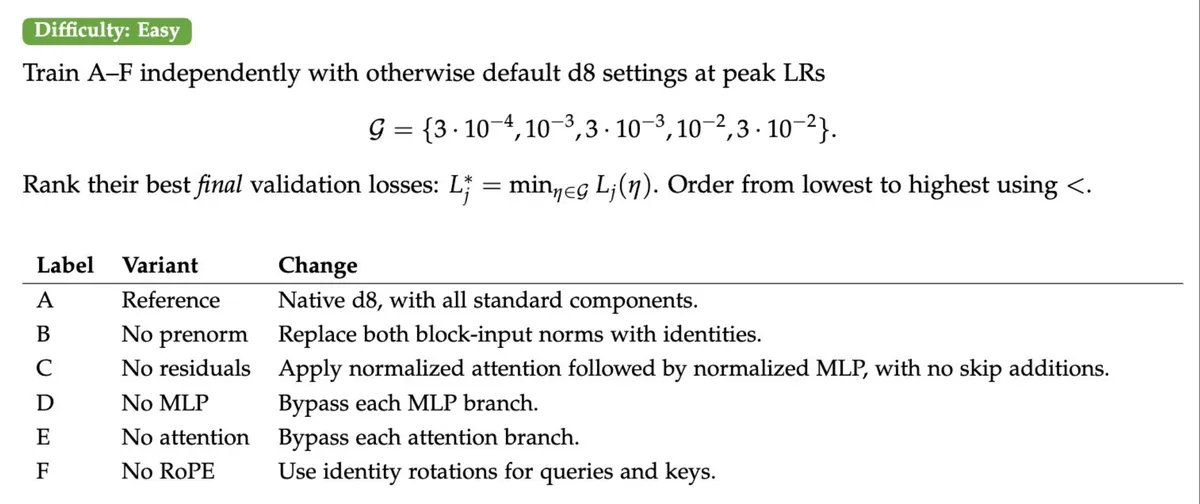
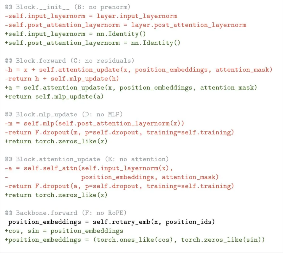
The full model is the natural baseline. It contains attention to mix information across tokens, an MLP to transform token representations, positional information, normalization, and residual connections. The interesting question is not merely which modification hurts the model most, but why.

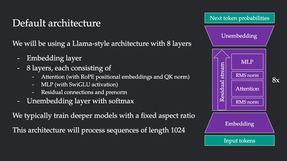
Consider removing PreNorm while keeping the residual connections. It is tempting to say that the hidden states will explode and training must fail. That conclusion is too strong. We can instead understand precisely what normalization changes, then distinguish the mathematical facts from an empirical prediction about validation loss.

A token's hidden representation is a vector of dimension $d$. Every nonzero vector can be separated into a length and a direction:

For example, if $h=[3,4]$, then its length is $5$ and its unit direction is $u=[0.6,0.8]$. The vector $[9,12]$ points in exactly the same direction but is three times longer. Should attention suddenly behave very differently just because the residual stream has become three times larger? Not necessarily: the relative pattern of features has not changed.

RMSNorm attempts to reduce this particular sensitivity. Its actual definition is

Here $\gamma$ contains learned per-coordinate gains, $ϵ$ avoids division by zero, and $\odot$ denotes elementwise multiplication. To see its geometry, temporarily ignore $\gamma$ and $ϵ$. Then

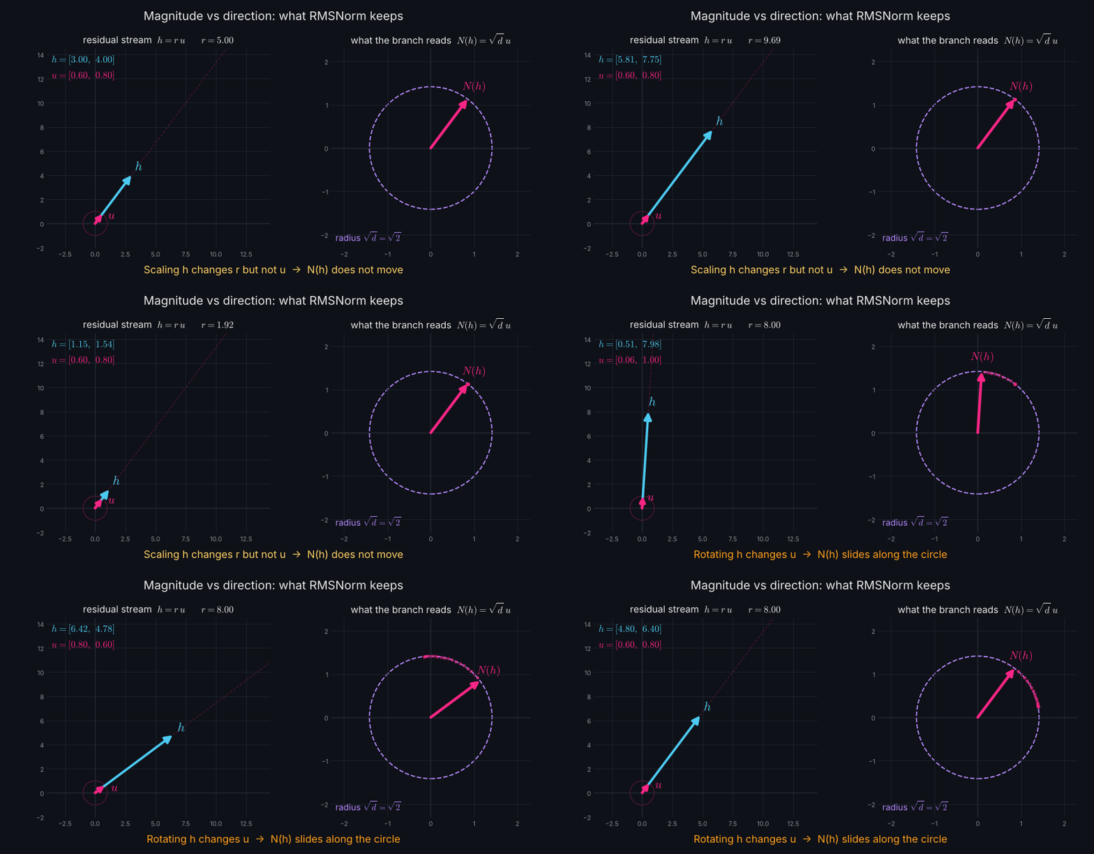
The simplified operation maps inputs of different positive scales to the same vector of length $\sqrt{d}$. In particular, for positive $c$,

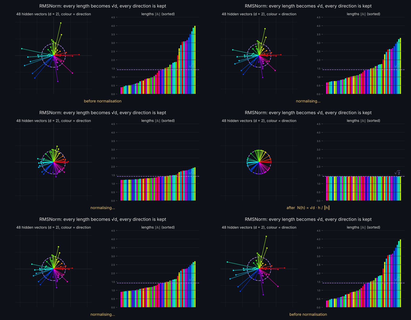
This identity is exact in the simplified model and only approximate with nonzero $ϵ$; nonuniform learned gains can also alter the output direction.

Recollect: magnitude versus direction. Any nonzero vector can be written as $h=ru$. The scalar $r$ is its length; the unit vector $u$ is its direction. Idealized RMSNorm removes the overall positive input scale while retaining the direction, up to a fixed multiplier.

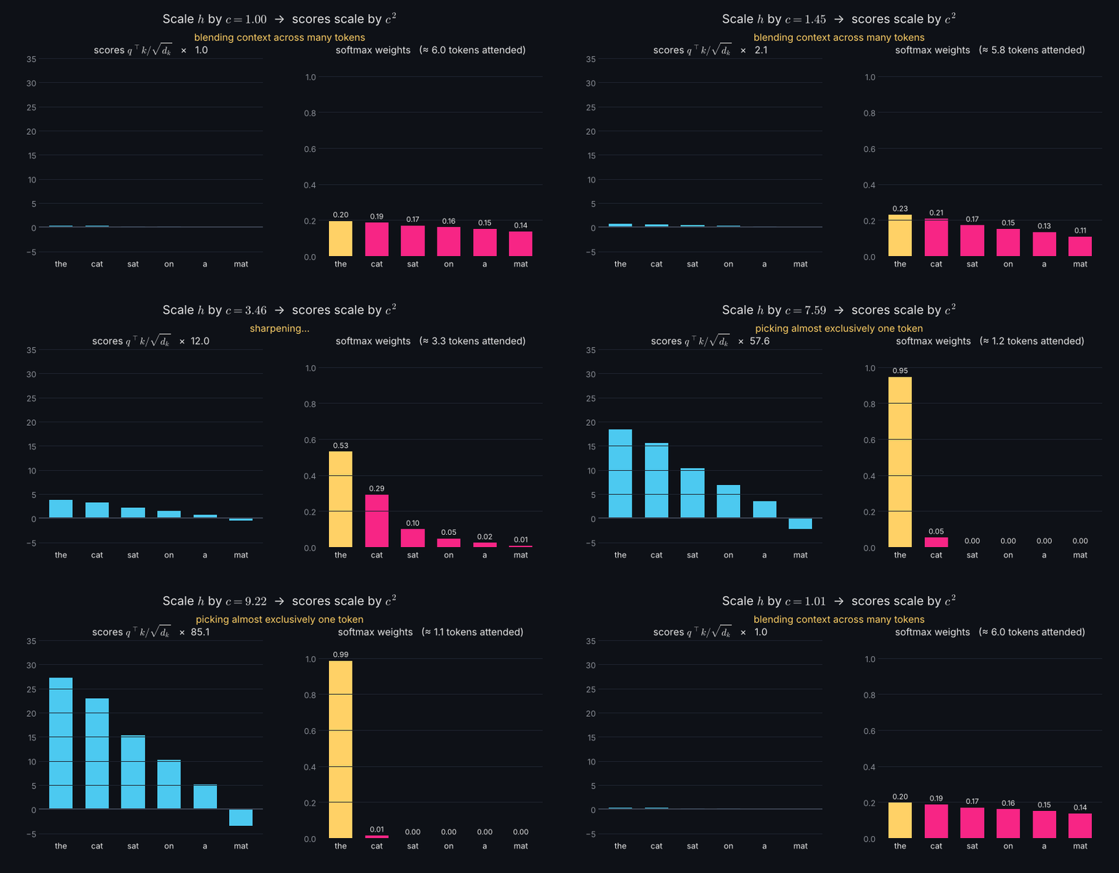
Why is scale important for attention? Recall the score between tokens $i$ and $j$:

Assume linear query and key projections without biases or extra query-key normalization. If both relevant input vectors become ten times larger, their queries and keys also become ten times larger, so the attention score becomes one hundred times larger:

Softmax is sensitive to this and if the Scores of $[1,2]$ produce probabilities of about $[0.269,0.731]$. Scores of $[10,20]$ produce probabilities of about $[0.000045,0.999955]$. Their ordering did not change, yet the computation went from combining two sources to selecting almost exclusively one. RMSNorm helps make the input scale seen by attention and MLP branches more predictable. It does not make them completely insensitive to all changes in their inputs.

The positioning of normalization matters as much as its presence. A simplified PreNorm residual branch is

The learned operation $F_l$ reads a normalized view of the current state. Separately, the unnormalized state $h_l$ continues directly through the residual path. This means the branch receives a scale-controlled input without forcing the entire residual stream to be normalized after each update. The stream remains free to evolve in both magnitude and direction.

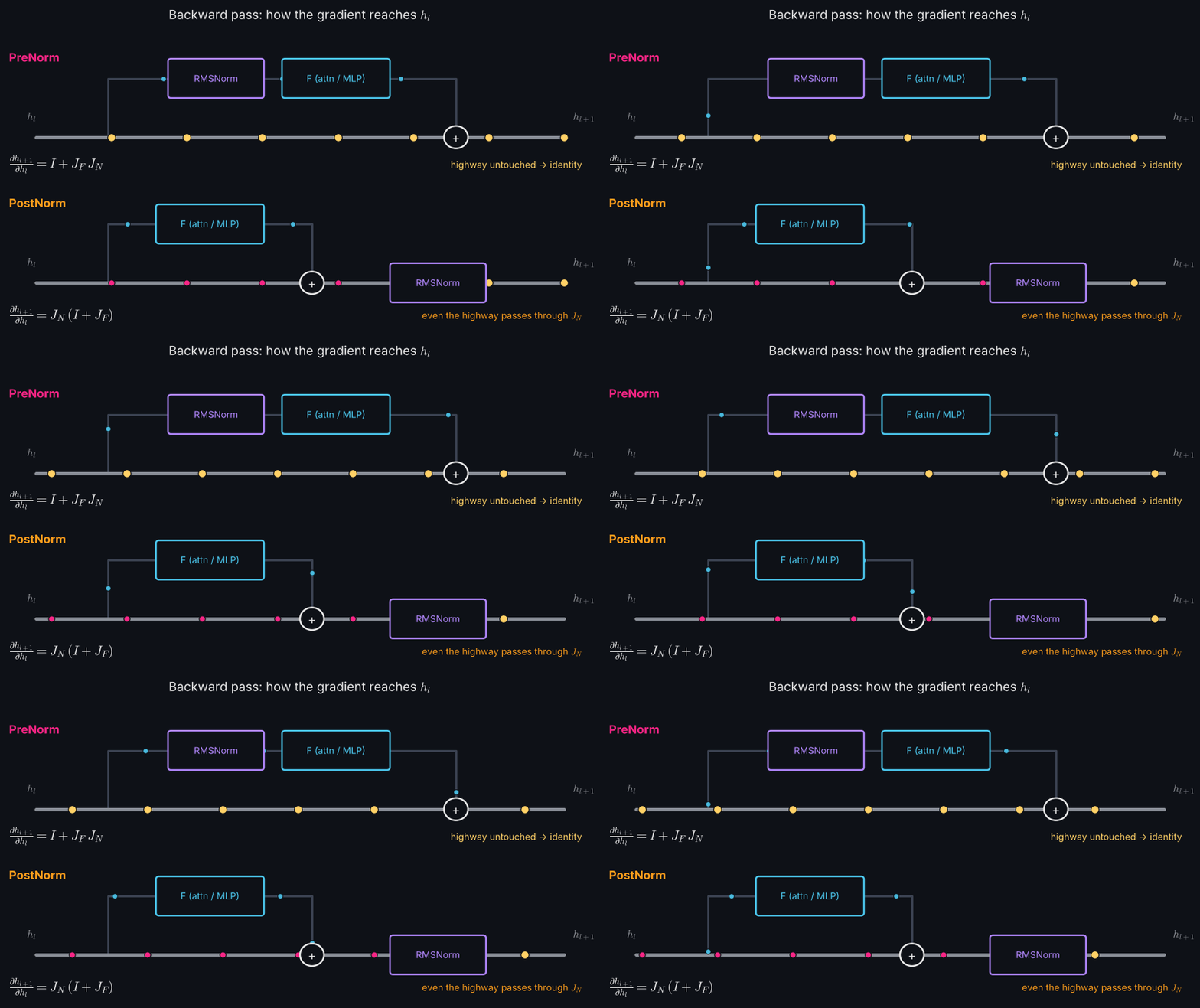
Recollect: two different jobs. PreNorm controls the input read by the branch. The residual connection preserves the direct path carrying the state forward. Removing either one changes a different part of the computation.

The same separation matters for gradients. The Jacobian of the PreNorm block, using the chain rule, is

The identity term $I$ is contributed by the direct residual path. It provides a local route through which changes and gradients can propagate without traversing every branch transformation. This does not guarantee perfectly stable gradients across an arbitrarily deep model, but it changes the optimization problem in a useful way.

In conventional PostNorm, normalization is applied after the residual addition:

and the Jacobian becomes

Now even the direct residual contribution passes through the normalization Jacobian. This helps explain why PreNorm is often easier to optimize at depth, though PostNorm can also work with suitable training choices.

If we remove PreNorm but retain residual connections, the branch becomes

Notice what remains: the existing representation still passes directly to the next layer, and the Jacobian still contains an identity contribution. What disappears is the branch's explicit protection from changes in residual-stream scale.

A toy model illustrates the distinction. Suppose every layer computes the update $F(h)=0.1h$. Without normalization,

After sixteen steps, the state is about $4.595$ times its starting value. Each new update is larger because it reads the accumulated state of the preceding layer.

For comparison, take a positive scalar input, idealized RMSNorm $N(h)=1$, and the same branch rule applied to the normalized input. Then

If $h_0=1$, the final value is $2.6$. In this narrow example, normalization changes repeated proportional updates into repeated constant updates. But this is not a general law of transformers. Learned branches can amplify, shrink, rotate, or cancel parts of the state. Neither exponential growth nor instability follows automatically from removing PreNorm.

Recollect: two recurrences. If every update is proportional to the current state, $h_{l+1}=(1+\alpha )h_l$ and the result compounds as $(1+\alpha {)}^L{h}_0$. If every update is a constant $c$, then $h_L=h_0+Lc$. Normalization reduces one path by which residual magnitude directly controls branch input, but it does not promise constant updates or bounded states in real networks.

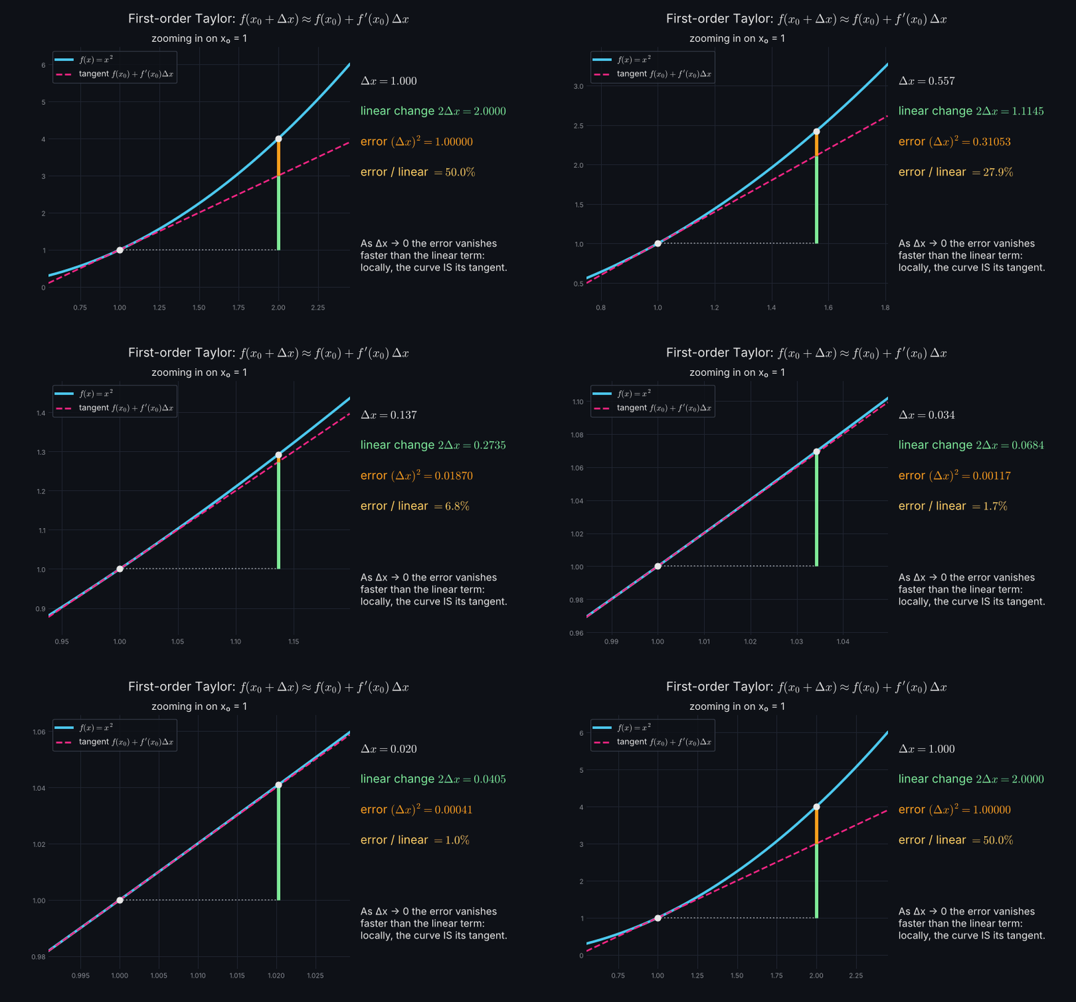
There is a deeper geometric way to understand the normalization operation: differentiate it. If $h$ changes a little, how much does $N(h)$ change? A derivative answers that question. For a scalar function $f(x)=x^2$,

For small $\Delta x$, the squared term is comparatively tiny, so

This is the first-order Taylor approximation. A smooth curve behaves locally like its tangent line. A vector-valued function behaves locally like a linear transformation, represented by the Jacobian matrix:

Now consider a vector-valued function:

A small input perturbation is

Unlike a scalar function, each output can depend on multiple input coordinates. We therefore use partial derivatives:

We can collect the partial derivatives into a matrix called the Jacobian:

Multiplying this matrix by the input change gives:

Notice that these are exactly the first-order changes we calculated for both output coordinates.

Therefore, we can write the entire approximation compactly as:

Recollect — The Jacobian as a local linear transformation

In one dimension, $f^{\prime }(x)\Delta x$ predicts the output change caused by a small input change.

In multiple dimensions, $J_F(h)\Delta h$ does the same thing, accounting for how every input coordinate influences every output coordinate.

Geometrically, the Jacobian transforms a small arrow in input space into the corresponding approximate arrow in output space.

The approximation becomes increasingly accurate as the perturbation approaches zero, provided the function is differentiable.

We can derive the Jacobian of idealized RMSNorm without memorizing a matrix-calculus formula. Write

First, square the length:

Recollect: familiar calculus rules. The product rule is $(ab{)}^{\prime }=a^{\prime }b+a{b}^{\prime }$. The quotient rule is $(a/b{)}^{\prime }=(b{a}^{\prime }-a{b}^{\prime })/b^2$. Matrix calculus applies these same principles while respecting multiplication order and dimensions. The expression $h^{\top }h$ is simply the sum of squared coordinates.

Differentiate both sides using the ordinary product rule:

The two dot products are the same scalar, so

Geometrically, the first-order change in a vector's length depends only on how much of the displacement points along the vector's current direction.

Imagine a vector as an arrow extending from the origin. There are two fundamentally different ways we can move its endpoint.

If we move along the arrow's direction, we are either stretching or shortening it. Its length changes immediately, in direct proportion to the displacement. This is the parallel component of the movement.

Suppose we move the endpoint of a vector perpendicular to its original direction, or sideways. Intuitively, we are not directly stretching the vector outward. Instead, we are primarily changing the direction in which it points.

But something interesting happens: the vector's length still increases, just by a much smaller amount than the sideways displacement itself. Why?

Imagine a vector of length $r=5$. We move its endpoint sideways by a small distance $ϵ$, perpendicular to the original vector.

By the triangle rule, the new vector is the sum of the original vector and this perpendicular displacement. Since the two vectors are perpendicular, they form a right triangle. The original vector is one side of length $r$, the sideways displacement is another side of length $ϵ$, and the new vector is the hypotenuse.

By the Pythagorean theorem,

Taking the square root,

Now, the important question is: How much longer has the vector become?

The change in length is

Substituting,

We can understand this without immediately using a Taylor expansion. Multiply and divide by the conjugate:

Using the identity $(a-b)(a+b)=a^2-b^2$, the numerator simplifies:

Therefore,

This expression is exact. We haven't approximated anything yet.

Now suppose $ϵ$ is very small compared with $r$. The new length will be very close to the original length:

So the denominator becomes approximately $2r$, giving

This is precisely the result we would obtain from a Taylor expansion:

Recall the first-order approximation

when $x$ is small. Substituting $x={ϵ}^2/r^2$,

Both approaches tell us the same thing.

Let's put some numbers into this.

Our original vector has length $r=5$. Suppose we move its endpoint sideways by $ϵ=0.1$.

The new length is

We moved the endpoint by $0.1$, but the vector's length increased by only about $0.001$.

Now halve the sideways displacement to $ϵ=0.05$.

The length now increases by only about $0.00025$, roughly one-fourth of the previous increase.

Why one-fourth? Because the change in length is proportional to the square of the sideways displacement:

If we halve $ϵ$, its square becomes one-fourth as large. If we make $ϵ$ ten times smaller, the increase in length becomes approximately a hundred times smaller.

This is what mathematicians mean when they say that a perpendicular displacement changes the vector's length only at second order.

To understand the distinction, recall that a first-order change is proportional to $ϵ$, whereas a second-order change is proportional to ${ϵ}^2$. As $ϵ$ approaches zero, ${ϵ}^2$ approaches zero much faster.

We can also see this directly from calculus. Define the length as a function of the sideways displacement:

Differentiating with respect to $ϵ$,

At the instant we begin moving sideways, $ϵ=0$, so

The first derivative is zero! This tells us that an infinitesimally small perpendicular movement produces no first-order change in length.

But the length is not perfectly constant. The second derivative at $ϵ=0$ is $1/r$, which gives the leading quadratic term ${ϵ}^2/(2r)$.

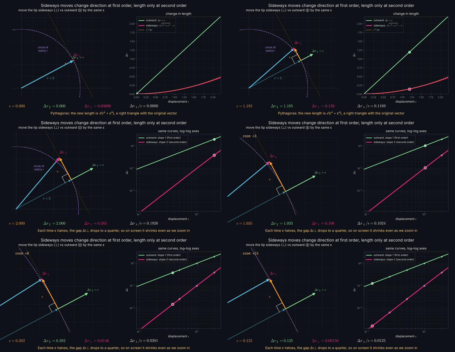
Geometrically, this makes sense. Moving directly along a vector immediately stretches or shortens it. Moving sideways initially changes its direction, and only gradually increases its length as the new endpoint moves away from the original circle of radius $r$.

This is also the intuition behind the derivative of vector normalization. If we normalize a vector, we deliberately remove its magnitude and retain its direction. A small displacement parallel to the vector changes only its magnitude, so normalization ignores it. A small perpendicular displacement changes its direction, so normalization responds to it at first order.

The deeper insight is that length and direction respond differently to movement. A radial displacement changes length at first order, while a perpendicular displacement changes direction at first order and length only at second order.

That distinction is exactly what appears in the Jacobian of RMSNorm.

It also explains the derivative we derived earlier:

Here, $u$ is the unit vector pointing along the original direction of $h$, and $dh$ is a small displacement. The dot product $u^{\top }dh$ measures the signed component of that displacement along $u$.

If the displacement is parallel, the dot product captures its full signed length. If it is perpendicular, the dot product is zero, meaning there is no first-order change in magnitude.

When we say that a perpendicular displacement produces no first-order change in magnitude, we are not saying that the vector's length does not change at all. We are saying something more precise: the length changes so slowly near the starting point that its change has no term proportional to the displacement itself.

To understand this, recall what a derivative measures. If we have a function $f(x)$ and make a small change $\Delta x$, its output can be approximated by

The term $f^{\prime }(x)\Delta x$ is called the first-order change because it is proportional to the displacement $\Delta x$.

For example, if $f^{\prime }(x)=3$, then a small displacement of $0.01$ produces an output change of approximately $0.03$. Halving the displacement approximately halves the change. This is characteristic of first-order behavior.

But what happens if the derivative is zero?

Then the first-order approximation becomes

This does not necessarily mean the function is perfectly constant. It means the function is locally flat to first order, and we must examine smaller, higher-order terms to understand how it changes.

Now consider our vector $h$, whose length is

Suppose we perturb it by a small vector $dh$. We previously derived that the first-order change in its length is

where $u=h/r$ is the unit vector pointing in the direction of $h$.

Recall the geometric interpretation of the dot product:

Since $u$ has unit length,

If the displacement is parallel to $h$, then $\theta =0^{\circ }$ and $\cos \theta =1$. Therefore,

The entire displacement contributes to the change in length. Moving outward by $0.1$ increases the length by $0.1$.

But if the displacement is perpendicular to $h$, then $\theta ={90}^{\circ }$ and $\cos \theta =0$. Therefore,

This means that the linear contribution to the change in length is zero. The sideways movement does not immediately stretch the vector in its existing direction.

However, for a finite perpendicular displacement of size $ϵ$, the Pythagorean theorem gives

And, as we derived earlier,

Notice the difference: the length still increases, but its leading change is proportional to ${ϵ}^2$, not $ϵ$.

For a concrete example, suppose $r=5$ and we move sideways by $ϵ=0.1$. The length increases by approximately $0.001$. If we halve the sideways movement to $0.05$, the increase becomes approximately $0.00025$—one-fourth as large.

So when we say there is no first-order change, we mean that the coefficient of the linear term is zero. The first nonzero contribution appears at second order.

This is an important distinction: the derivative tells us what happens infinitesimally, not that every finite movement leaves the length unchanged.

Geometrically, a perpendicular displacement initially moves the endpoint along the tangent direction of the circle centered at the origin. The tangent is perpendicular to the radius, so the movement initially changes the vector's direction rather than its distance from the origin. Only as we move a finite distance along that tangent does the endpoint move farther away from the circle.

In short, a parallel displacement changes the vector's length immediately, at first order. A perpendicular displacement changes its direction immediately, while its length increases only at second order. This is why the dot product with the unit direction vector captures exactly the first-order change in magnitude.

Recollect — The geometric meaning of $dr=u^{\top }dh$

The derivative measures how quickly the vector's length changes under an infinitesimal displacement.

• Parallel movement: changes the length at first order.
• Perpendicular movement: changes the direction at first order, but the length only at second order.

The fundamental insight is that the first-order change in magnitude is exactly the projection of the displacement onto the vector's current direction.

Next, differentiate the unit direction $u=h/r$ by treating $r$ as a scalar denominator:

Substitute $dr=u^{\top }dh$ and $h=ru$:

Because $u(u^{\top }dh)=(u{u}^{\top })dh$ and $dh=Idh$,

Finally $N(h)=\sqrt{d}u$, giving

Hence the Jacobian is

Why does the matrix $I-u{u}^{\top }$ appear? The answer comes from projection, one of the most useful geometric ideas in linear algebra.

Take a unit vector $u=[0.6,0.8]$ and another vector $v=[5,0]$. The dot product is

For a unit vector, $u^{\top }v=\Vert v\Vert \cos \theta$ is the signed length of $v$'s shadow along $u$. The dot product gives a number, not a vector. Multiply by the unit direction to reconstruct the parallel vector:

The perpendicular remainder is

We can check that it is perpendicular:

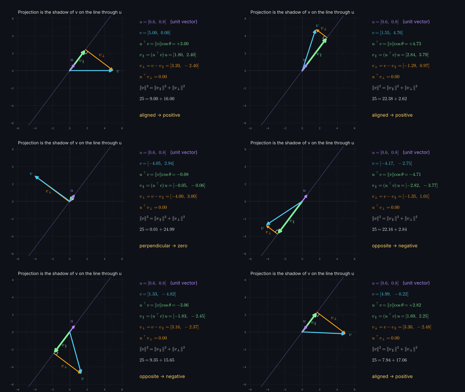
This is the triangle law: $v=v_{\parallel }+v_{⟂}$. Place the parallel and perpendicular displacements head-to-tail; together they reproduce the original vector. The dot product tells us how much of the vector lies along $u$, and subtraction gives the remainder.

Recollect: the dot product. The notations $u^{\top }v$ and $u·v$ mean the same operation. In general, $u^{\top }v=\Vert u\Vert \Vert v\Vert \cos \theta$. For unit $u$, the dot product $u^{\top }u=\Vert u{\Vert }^2=1$. A zero dot product means perpendicular vectors.

We can rewrite projection as a matrix operation. First measure the scalar $u^{\top }v$, then reconstruct the vector by multiplying by $u$:

Thus $u{u}^{\top }$ is a projection matrix. Importantly, $u^{\top }u$ is a scalar, while $u{u}^{\top }$ is a matrix. Their multiplication order makes them fundamentally different.

Subtracting the projection from the original vector gives

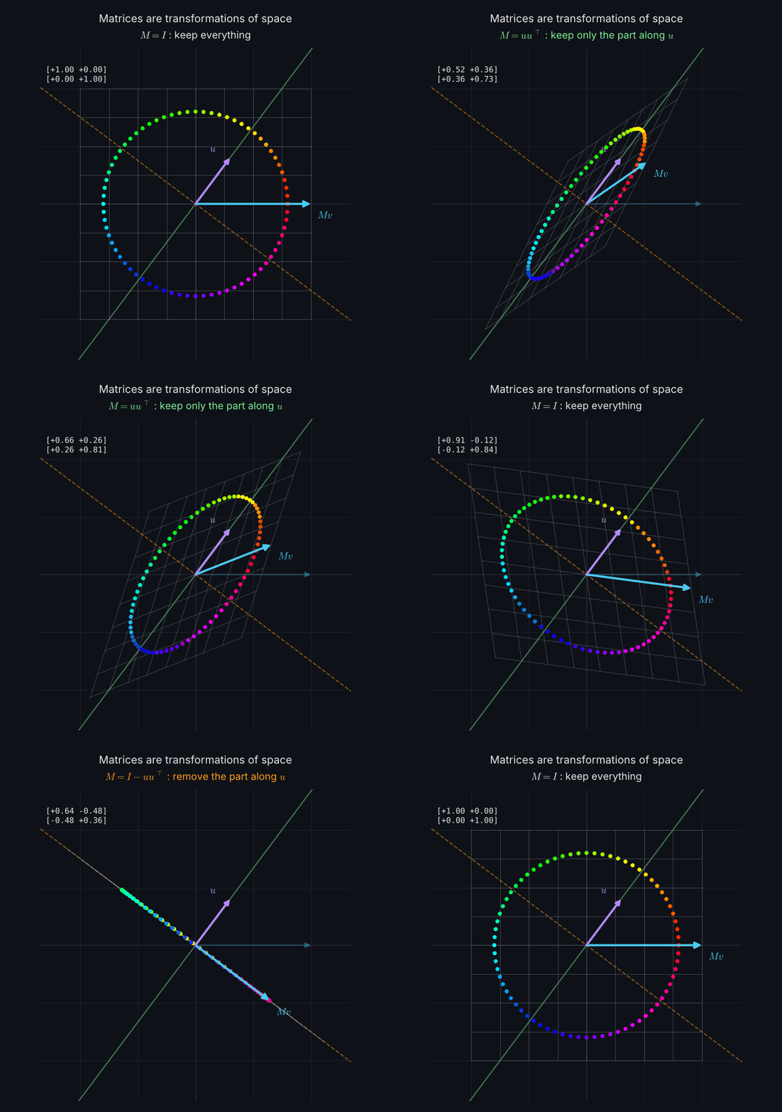
In other words, $u{u}^{\top }$ keeps the component along $u$, while $I-u{u}^{\top }$ keeps the component perpendicular to $u$. This explains every term in the normalization Jacobian:

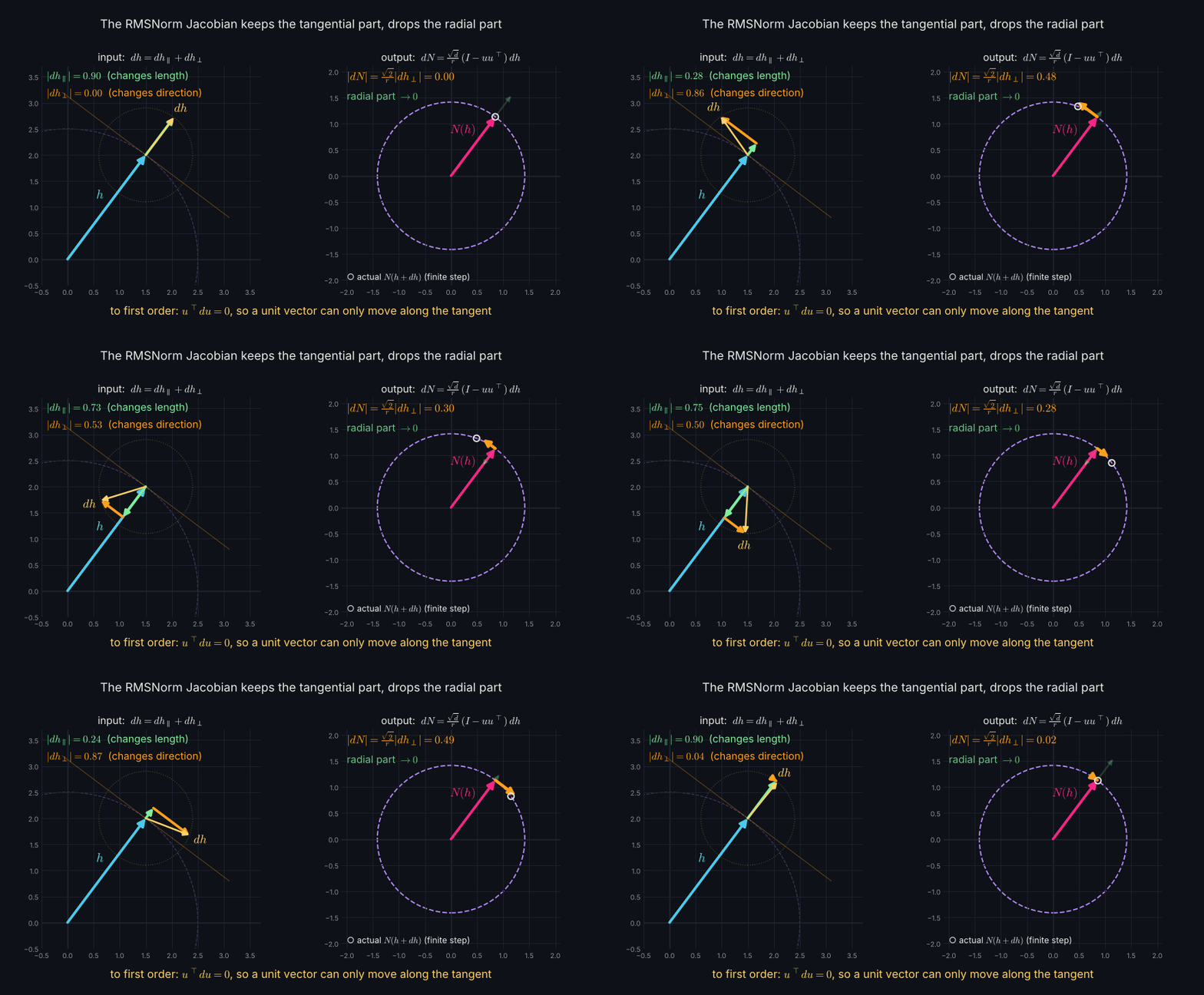
Idealized normalization discards the first-order radial change and reacts to changes of direction. If we double $h=[3,4]$ to $[6,8]$, its normalized direction stays exactly the same. In Jacobian language, $J_N(h)u=0$. But a small sideways displacement changes its direction, so the Jacobian preserves and rescales that perpendicular component.

There is a shorter proof of the same geometry. Since the normalized direction always has unit length,

Differentiate:

Both terms are equal scalars, so

An infinitesimal movement of a unit vector must be perpendicular to the unit vector itself. In two dimensions the normalized output travels along a circle, and its instantaneous movement lies on the circle's tangent. In higher dimensions it lies in the tangent plane of a sphere. A finite chord between two points is not necessarily perpendicular to the original radius; the statement applies to the infinitesimal derivative.

Recollect: the geometry of the Jacobian. The factor $I-u{u}^{\top }$ removes a perturbation's component along the current direction. The factor $\sqrt{d}/r$ rescales the remainder. Therefore idealized RMSNorm's derivative responds to changes in direction, not pure positive rescaling. Actual RMSNorm has $ϵ$ and learned gains, so the exact Jacobian differs.

This brings us back to PreNorm. The normalized branch receives a standardized view of the state, but the residual path does not pass through that normalization. In the simplified model, a radial perturbation $u$ satisfies $J_{N}u=0$, while the whole PreNorm block has

The branch is locally insensitive to that pure scaling direction; the direct residual path still carries it onward. This illustrates a useful division of responsibilities, not a guarantee that every piece of information survives through the full trained network.

With this mental model, removing PreNorm is not automatically catastrophic. It makes the learned branches more sensitive to variations in the residual stream's scale but leaves their computational mechanisms and direct state path intact. In a relatively shallow transformer, suitable initialization, parameters, and training settings may be enough for the model to remain competitive. How much performance changes is an empirical question, not something the algebra can settle by itself.

The practical test of the normalization explanation is to inspect residual-stream RMS, attention-logit distributions, activations, and gradient norms across layers. If a model without PreNorm remains well behaved on these quantities, there is no mathematical reason it must fail. If they drift or become unstable, they provide clues about the mechanism of failure.

The deeper lesson is about building a predictive mental model rather than memorizing which component is more important. Magnitude and direction explain normalization. Dot products and projections explain its geometry. Jacobians explain local sensitivity. Residual connections explain the direct state path. These ideas fit together into one design intuition: