what even are diffusion models doing ? - part-1

25 Jun, 2026

let’s assume we have a prompt and we want to generate some data from it. that data could be an image, audio, video, protein structure, or whatever. but for simplicity, let’s understand everything with images.

Diffusion forward and reverse process

assume we want to generate an image vector $x$ . to keep the story simple, let’s say we want one image vector for a given prompt $p$ .

at a very informal level, we might say:

x = f (p)

where $p$ is the prompt.

but technically, this is not quite right. a prompt does not usually map to only one fixed image. if i say:

a cat holding a banana

there are infinitely many valid images that could satisfy that prompt. the cat could be orange, black, realistic, cartoonish, sitting, standing, indoors, outdoors, and so on.

so the better way to think about it is not:

x = f (p)

but rather:

x ~ p_{d} (x ∣ p)

this means: sample an image $x$ from the real distribution of images that match prompt $p$ .

so the job of the model is to learn an approximation:

p_{θ} (x ∣ p) \approx p_{d} (x ∣ p)

where $p_{d}$ is the real data distribution and $p_{θ}$ is the model distribution learned by the neural network.

The big goal

neural networks are universal function approximators. so we hope the model can learn a very complicated mapping from prompts and random noise to realistic data.

in a sense, we want the model parameters $θ$ to capture the distribution of possible images: cats, bananas, humans, cars, lighting, textures, compositions, rare combinations, and even weird stuff like:

a cat holding a banana and dipping it in liquor

the exact event may be extremely rare in the real world. its probability under the real data distribution may be tiny. but if the model has learned the concepts of “cat,” “banana,” “holding,” “dipping,” “glass,” and how objects interact visually, then it can still generate a plausible sample from:

p_{θ} (x ∣ "cat holding a banana and dipping it in liquor")

so the model is not just memorizing exact images. it is learning the structure of the image distribution and how language conditions that distribution.

Direct probability matching

the first natural idea is: let’s directly make the model distribution close to the data distribution.

we have:

p_{d} (x)

for the real data distribution, and:

p_{θ} (x)

for the model distribution.

the dream is:

p_{θ} (x) \approx p_{d} (x)

or in the prompt-conditioned case:

p_{θ} (x ∣ p) \approx p_{d} (x ∣ p)

so we can imagine designing a loss function that measures the mismatch between these two distributions:

ℒ (θ) 𝔼_{p_{d} (x)} [\frac{1}{2} {| p_{θ} (x) - p_{d} (x) |}^{2}]

the intuition is simple: if the model distribution is far from the real data distribution, the loss is high. if the model distribution matches the real data distribution, the loss is low.

training means changing $θ$ so that the model’s imagination gets closer to reality.

The problem: probability is too hard

here comes the problem.

estimating the probability of data directly is basically impossible for high-dimensional data like images. a single image is already a massive vector. the number of possible images is beyond imagination.

still, mathematically, we can write a very general model distribution using an energy function:

p_{θ} (x) = \frac{1}{Z (θ)} e^{- ℰ_{θ} (x)}

here, $ℰ_{θ} (x)$ is the energy assigned to image $x$ .

low energy means the model thinks the image is realistic.

high energy means the model thinks the image is unrealistic.

the negative sign makes sense:

e^{- ℰ_{θ} (x)}

if the energy is low, this value is high. if the energy is high, this value is low.

so minimizing energy is like maximizing probability.

but this expression needs a normalizing factor:

Z (θ)

because probabilities must integrate to $1$ .

the normalizing constant is:

Z (θ) = \int_{y} e^{- ℰ_{θ} (y)}, d y

i am using $y$ instead of $x$ here to make the meaning clearer.

this integral says: go over every possible image $y$ , compute its unnormalized score $e^{- ℰ_{θ} (y)}$ , and add everything together.

so the actual probability is:

p_{θ} (x) = \frac{e^{- ℰ_{θ} (x)}}{\int_{y} e^{- ℰ_{θ} (y)}, d y}

the numerator asks:

how good is this specific image $x$ ?

the denominator asks:

what is the total score of all possible images?

and this is where things break.

computing $Z (θ)$ is intractable because we cannot sum over all possible images. there are simply too many possible $x$ ’s.

Autoregressive route

one way around this is the autoregressive way.

in autoregressive models, we break data into pieces and model the joint probability as a product of conditional probabilities:

p (x_{1}, x_{2}, \dots, x_{n}) = p (x_{1}) p (x_{2} ∣ x_{1}) p (x_{3} ∣ x_{1}, x_{2}) \dots p (x_{n} ∣ x_{1}, \dots, x_{n - 1})

this is basically what llms do with text. instead of modeling the full sequence all at once, they predict the next token given the previous tokens.

but diffusion takes another route.

Diffusion route: remove the normalizing constant ><

the diffusion route says: instead of directly computing the probability $p_{θ} (x)$ , look at the gradient of the log probability with respect to the data:

\nabla_{x} \log p_{θ} (x)

this is called the score.

start from the energy-based model:

p_{θ} (x) \frac{1}{Z (θ)} e^{- ℰ_{θ} (x)}

take log:

\log p_{θ} (x) = - \log Z (θ) ℰ_{θ} (x)

now take gradient with respect to $x$ :

\nabla_{x} \log p_{θ} (x) = \nabla_{x} [- \log Z (θ) ℰ_{θ} (x)]

since $Z (θ)$ depends on the model parameters $θ$ , not on this particular input $x$ , we get:

\nabla_{x} \log Z (θ) = 0

so:

\nabla_{x} \log p_{θ} (x) = - \nabla_{x} ℰ_{θ} (x)

this is the beautiful trick.

the intractable normalizing constant disappears.

so instead of matching probabilities directly:

p_{θ} (x) \approx p_{d} (x)

we try to match score functions:

\nabla_{x} \log p_{θ} (x) \approx \nabla_{x} \log p_{d} (x)

the model score tells us something like:

if i slightly move this image vector $x$ , which direction makes it more likely under the model?

it is like an arrow pointing toward higher-probability, more realistic regions of image space.

But there is still a problem :(

we got rid of $Z (θ)$ , yes.

but we still do not know:

\nabla_{x} \log p_{d} (x)

because we do not know the real data distribution $p_{d} (x)$ .

we only have samples from it. we have images, but we do not have the formula for the probability landscape of real images.

so diffusion makes a clever detour.

Denoising detour

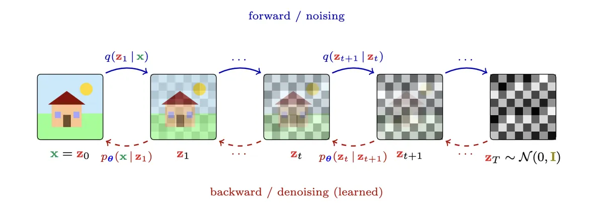
instead of trying to learn the clean data distribution directly, we create a known corruption process.

we take a real training image $x$ , add gaussian noise to it, and create a noisy image:

z_{t} = α_{t} x + σ_{t} ϵ

where:

ϵ ~ 𝒩 (0, I)

here, $t$ is the noise level or timestep.

the coefficient $α_{t}$ controls how much of the original image remains.

the coefficient $σ_{t}$ controls how much noise is added.

when $t$ is small:

α_{t} \approx 1, σ_{t} \approx 0

so:

z_{t} \approx x

the image is almost clean.

when $t$ is large:

α_{t} \approx 0, σ_{t} \approx 1

so:

z_{t} \approx ϵ

the image is almost pure gaussian noise.

so we have a forward process:

x \to z_{1} \to z_{2} \to \dots \to z_{T}

where $z_{T}$ is basically gaussian noise.

this noising process is mathematically easy because we designed it ourselves.

the hard part is learning the reverse:

z_{T} \to z_{T - 1} \to z_{T - 2} \to \dots \to x

Signal-to-noise ratio

one useful way to understand the noise level is through the signal-to-noise ratio, or snr. since the noisy image is written as:

z_{t} = α_{t} x + σ_{t} ϵ

the term $α_{t} x$ is the remaining real image signal, and the term $σ_{t} ϵ$ is the added noise. so the snr is:

{S N R}_{t} = \frac{α_{t}^{2}}{σ_{t}^{2}}

if ${S N R}_{t}$ is high, the image still contains a lot of real signal and only a little noise. if ${S N R}_{t}$ is low, the image is mostly noise and only a little signal. people often use the log-snr:

λ_{t} = \log {S N R}_{t} \log \frac{α_{t}^{2}}{σ_{t}^{2}}

because it is numerically easier to work with. in simple words, snr tells us where we are in the diffusion journey: high snr means close to the clean image, low snr means close to pure gaussian noise.

Training the model

during training, we take real image-prompt pairs:

(x, p)

we sample a random timestep $t$ .

we add noise:

z_{t} = α_{t} x + σ_{t} ϵ

then we give the model:

(z_{t}, t, p)

and ask it to predict the noise:

ϵ_{θ} (z_{t}, t, p) \approx ϵ

the loss is usually something like:

ℒ (θ) 𝔼_{x, p, t, ϵ} [{| ϵ_{θ} (z_{t}, t, p) - ϵ |}^{2}]

sometimes the model predicts the clean image $x$ , sometimes it predicts the noise $ϵ$ , and sometimes it predicts a velocity-like quantity $v$ .

but the core idea is the same:

the model learns how to denoise.

How this learns the data distribution

now the key question:

how does denoising approximate $p_{d}$ ?

if you take all real images:

x ~ p_{d} (x)

and you add gaussian noise at time $t$ , you get a new distribution:

q_{t} (z_{t}) = \int q_{t} (z_{t} ∣ x) p_{d} (x), d x

this is the distribution of noisy real images at noise level $t$ .

at $t = 0$ , this distribution is basically the real data distribution:

q_{0} (x) \approx p_{d} (x)

at large $t$ , this distribution becomes close to pure gaussian noise:

q_{T} (z_{T}) \approx 𝒩 (0, I)

so diffusion builds a bridge:

p_{d} (x) \to q_{t} (z_{t}) \to 𝒩 (0, I)

training teaches the model how to walk backward across this bridge.

if the model learns the reverse denoising direction correctly for every timestep, then at generation time we can start from pure noise:

z_{T} ~ 𝒩 (0, I)

and repeatedly denoise:

z_{T} \to z_{T - 1} \to z_{T - 2} \to \dots \to z_{0}

at the end, $z_{0}$ should look like a real image:

z_{0} ~ p_{θ} (x)

and ideally:

p_{θ} (x) \approx p_{d} (x)

in the prompt-conditioned case:

p_{θ} (x ∣ p) \approx p_{d} (x ∣ p)

The important intuition

the model is not learning one fixed mapping from one noisy image to one clean image.

for every image, there are infinitely many possible noisy versions because every noise sample $ϵ$ is different.

also, at high noise levels, one noisy point could be consistent with many possible clean images.

so this is not a one-to-one mapping.

what the model really learns is a denoising field:

given a noisy point $z_{t}$ , a time $t$ , and a prompt $p$ , which direction should we move to become more like realistic data matching that prompt?

you are giving the model billions of broken pictures that you broke in a mathematically controlled way.

then you ask it again and again:

what was the noise?

or:

how do i get back to the clean image?

after seeing enough examples, the model generalizes. it learns the structure of real images, the structure of language, and the relationship between prompts and images.

then at inference time, you give it pure noise plus a prompt, and it gradually sculpts the noise into an image that belongs to the learned conditional distribution.

Final picture

the final generation process is:

prompt p + noise z_{T} \to reverse diffusion \to image x

more formally:

z_{T} ~ 𝒩 (0, I)

z_{T} \to z_{T - 1} \to \dots \to z_{0}

z_{0} ~ p_{θ} (x ∣ p)

and the whole training goal is:

p_{θ} (x ∣ p) \approx p_{d} (x ∣ p)